Hacking Houdini Solaris Procedurals

I’ve long been fascinated with the possibilities provided by rendertime procedurals in going to the next level of complexity in 3D scenes.
In the past, I’ve worked with them for fur, fractals, oceans and clouds. Some years ago I even coded a 90%-finished Arnold-Houdini Engine procedural (back then that was in some sense the holy grail, but now barely relevant due to the advent of Solaris), which would’ve allowed taking an arbitrary HDA to generate geometry at rendertime.
In this post, I’ll explain some of the more arcane technical details of how Houdini Solaris procedurals work. I’ll also show how to not only build your own but also unpack and customize any existing procedural (something which as far as I know no other resource does).
“Very Esoteric” — How Solaris Procedurals Work
Invoke Graph and Node Networks as Geometry
“The Usefulness of This Node is Very Esoteric” – This line ends two terse paragraphs about the Invoke Graph node. It might also be the greatest line of text in all of Houdini’s massive documentation.
Invoke graphs are at the heart of most1 Solaris procedurals.
For some context, let’s start with compile blocks – an older and in some ways similar technology. Compile Blocks enclose a network of nodes, and are mainly used for For-Each Loops being executed in parallel (we’ll see an example of this below). The Invoke Compiled Block SOP allows you to execute an existing compile block with new inputs anywhere in your network. In programming terms, you can think of the Compile Block as a function and the Invoke Compiled… SOP as calling that function with different input geometries.
In Houdini 19, SideFX introduced the concept of encoding node networks as geometry, using the Attribute as Parameters SOP. This records nodes as points with attributes for the name, path, position, with edges/polylines between points encoding connections between the respective nodes. The Invoke Graph SOP then allows executing a graph that was previously converted to geometry in the same way as Invoke Compiled Block does for Compile Blocks.2
At first glance, this seems like a strange and indeed esoteric concept, but thinking about it, it allows you to use nodes to manipulate geometry that encodes a node network. This in itself is already interesting and brings to mind other coding concepts like Metaprogramming, Lisp Macros, and functional programming in general.
More commonly, you can also write out this geometry to a file and reuse it in a different scene without the overhead of a full HIP file or HDA.
Husk Procedurals
Husk is a program that comes with Houdini and is responsible for invoking a USD render delegate, such as Karma, Arnold or Renderman.
Here’s how Husk uses procedurals:
- the LOPs for each procedural create USD primitives with special attributes. These point to an arbitrary Python script (which, importantly, can use the
houPython API) - At rendertime, Husk runs this script and passes the resulting geometry to the render delegate
- Most procedurals use a script called
invokegraph.py, which is part of the the Houdini distribution.- It loads a graph (created by
attribfromparm) from a.bgeofile - It then runs the
invokegraphSOP3 on that - It puts the output into a new USD primitive
- It loads a graph (created by
These things together give you have all the ingredients for procedurals in a fairly elegant solution.
Further Resources
- Fuat Yüksel’s talk at FMX is a great resource and might help with understanding the use and internal functionality of procedurals.
- Paul Ambrosiussen (text version) provides some details that both the above talk and the documentation glance over
Creating your own procedurals
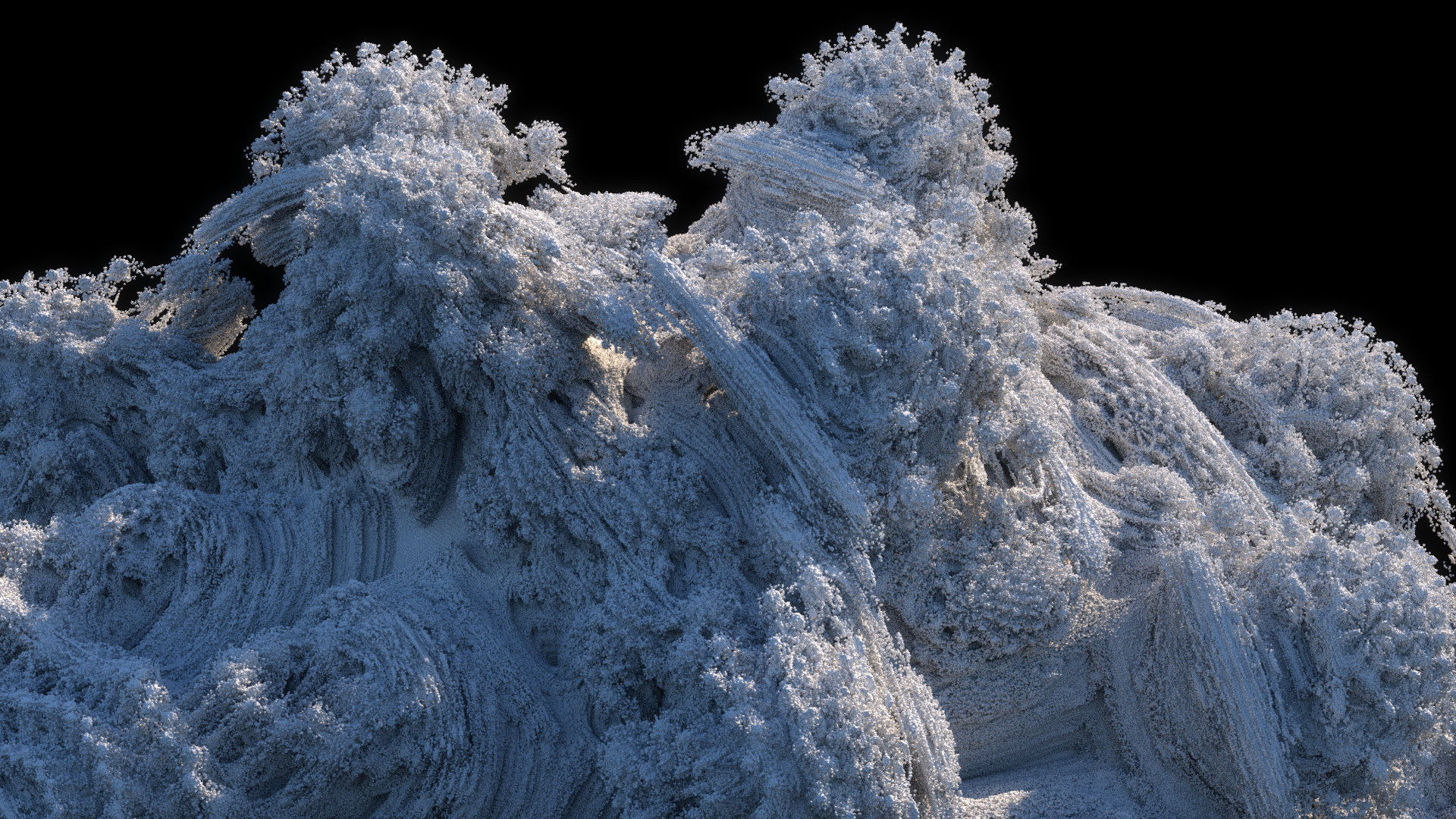
In this section, we’ll build our own procedural to generate a point-based Mandelbulb, in the tradition of the C++-based Arnold version.
The Arnold version not only involves quite a bit of boilerplate, but also requires you to have a working setup for compiling C++ with exactly the right compiler version, know about shared libraries, environment variables, have some knowledge of the Arnold SDK, and you also need to put your compiled procedural shared library in exactly the right place for Arnold to find it.
With the Houdini procedural approach, we can first prototype our procedural in Houdini (even running the graph directly with Invoke Graph for testing), then deploy it for the renderer to use, all while staying quite a bit simpler and able to iterate faster.
Basic Mandelbulb Setup
One of the easiest approaches to generating a Mandebulb is by checking each point in a dense grid for membership of the Mandelbulb set.
- To create the grid:
- use a
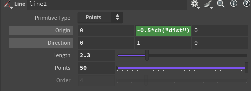
LineSOP of length $2.3$ and centered at 0 to create points on the y axis - use
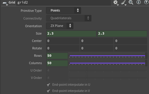
Copy to Pointsto copy aGridSOP of size $2.3$x$2.3$ in the x/z axes onto each point of the line.
- use a
- to check for each point’s set membership:
- run the Mandebulb iteration formula $Z=Z^n+C$ on each point
(starting with $Z_0=(0,0,0)$ and $C=P$) - Then check which points “escape” (ie their iterated position $Z$ moves more than a certain distance from away from $(0,0,0)$) and delete them.
- run the Mandebulb iteration formula $Z=Z^n+C$ on each point
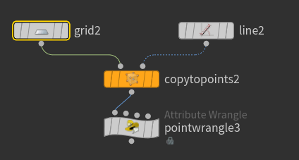
For the actual Mandelbulb sampling, we just use a pointwrangle SOP. The following code (in contrast to the Arnold sample) uses a spherical coordinate approach. This is not better or worse than other methods for this case, but I already had the relevant VEX code.
1
2
3
4
5
6
7
8
9
10
11
12
13
14
15
16
17
18
19
20
21
22
23
24
25
26
27
28
29
30
31
32
33
34
35
36
int mandelbulbSDF(const vector pos) {
    int iters = 30;
    float power = 8.0;
    float maxdist = 2;

    float r = 0.0;
    vector z = {0,0,0};
    for(int i=0; i<iters; ++i) {
        r = length(z);
        if(r > maxdist) {
            return false;
        }

        // to polar/spherical coords
        float theta = acos(z.z / r);
        float phi = atan(z.y, z.x);

        // apply iteration
        float zr = pow(r, power);
        theta = theta * power;
        phi = phi * power;

        // back from polar/spherical coords
        z = zr * set(sin(theta) * cos(phi), sin(phi) * sin(theta), cos(theta));

        z += pos;
    }
    return true;
}

if(! mandelbulbSDF(v@P)) {
    removepoint(geoself(), i@ptnum);
}
else {
	f@pscale = 0.005;
}
There’s plenty of writing on Mandelbulbs (and other 3D fractals) and their formulae, and how to best evaluate them, so I won’t elaborate on that topic too much here. The method used here is far from the most efficient, but is simple and effective for demonstrating how to set up procedurals.
The above should already be parallelized and use, e.g, SIMD sin/cos functions, thanks to the power of VEX. In my version, I also wrapped things in a For Each Block and a Compile block, to improve multithreading and memory use, along similar lines as the Breaking Generation into Chunks section in the above-linked Arnold example.
Wrapping it into a Procedural
As it’s a fairly simple procedural, we can just copy and adapt one of the existing procedurals coming with Houdini, which, for the most part, use invokegraph.py. In my tests, I used a mix of the feather and ocean procedurals.
The steps for converting the nodes that create our Mandelbulb to a procedural then are:
- Wrap the Mandelbulb generation nodes in a subnet
- Put down an
Attribute from ParametersSOP.- Set its Method to Points from Subnetwork
- Its Node Path to the subnet for the mandelbulb
- Enable Create Inputs and Outputs
- Add a blast node, set its
group typeto Points and the group to1-3or@name==__input1 @name==__input2 @name==__input3. That way,invokegraphwill not complain about missing inputs. (The remaininginput0input is for adding parameter overrides, see next section.) - Write out the result to a
.bgeofile using aFileorFile Cachenode - In LOPs, create a subnetwork for the procedural and add an adapted version of the define_and_setup_hair_deform_procedural node from within the
houdinifeatherproceduralnode. The adjustments are fairly obvious in that you need to ensure your.bgeo.scfile from the previous step is used as the graph and the right attributes/parameters are passed to it - Test with a
houdinipreviewproceduralLOP
Making the procedural adjustable
As the invokegraph documentation mentions, channel references and other HScript expressions don’t work with it. There’s a mention of “parameter overrides” as a solution to the problem, unfortunately without any further explanation (or mention in the docs that I could find).
Parameter overrides work by taking a parms dictionary detail attribute on a given override node and use their values to override corresponding parameter values on any node. To create that dictionary, the Attribute Adjust Dictionary SOP can be used.
- Add a new spare input on the node whose parameters should be overridden
- drag the node with your dictionary in there.
- To tell Houdini to use the parameter overrides, create an extra integer parameter called
spare_parminputindexand set it to the corresponding spare parm input number (starting at $-1$ for spare input $0$, then $-2$ etc, exactly like in VEX). - On doing so, your spare parm’s network connection (usually a dashed line) will change color, and the override gets used.
Here’s a simple example with a cube whose length in x gets overwritten by a dictionary:
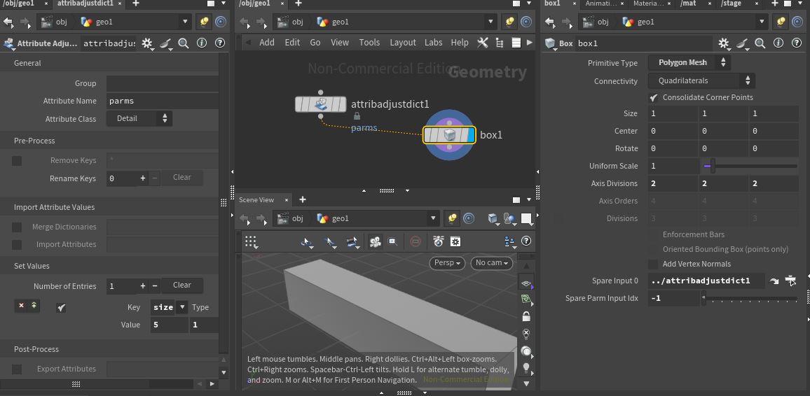
attributeadjustdict node by adding an entry of $(5,1,1)$ of type vector for the size attribute .Parameter overrides on procedurals work in the same way. The invokegraph.py script passes overrides as an input geometry to the procedural, where they can then be used to tweak things.
Unpacking and customizing existing procedurals
In production scenarios you might want to customize existing procedurals, whose core functionality is often only available as a geometry representation in a bgeo file rather than a Houdini scene or HDA.
I’ve spent some hours implementing a Python script that converts the output of Attribute from Parameters as used in Houdini’s own procedurals back to a node graph.
(It still has some minor missing features and requires cleanup, so I’m not sharing it yet, but feel free to contact me if you’re interested.)
Here are some examples of the converted procedurals.
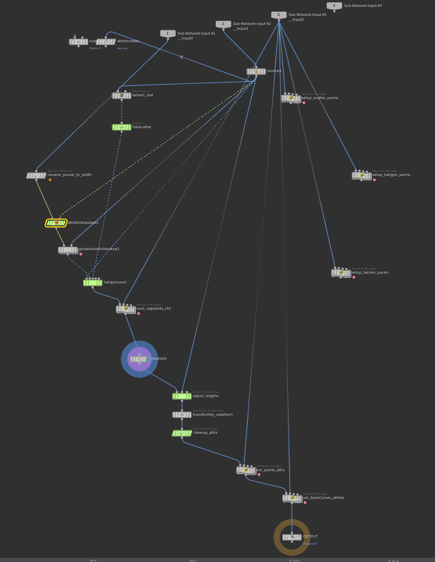
The network for the Solaris hair procedural
The network for the Solaris ocean procedural is actually a compile block!

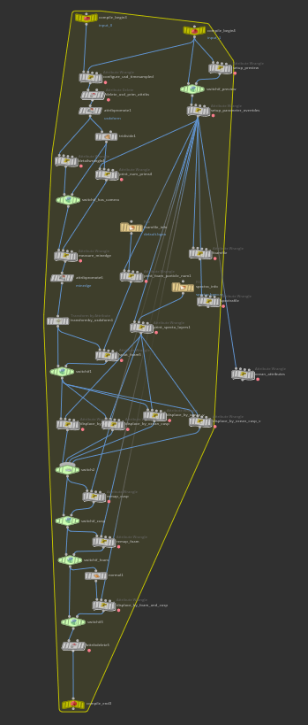
The network for the feather procedural. It provides a good example of how overrides are used.
More results
If your studio needs any help with Houdini procedurals or other FX/technical tasks I’m available for freelance - hit me up via e-mail or on LinkedIn.
-
One exception from this is the crowds procedural, as it doesn’t use this geometry-as-graphs approach. Digging into it reveals that it ends up calling some custom C++ code, but to do so, it uses the same Python wrapper approach described above. ↩
-
Internally,
Invoke Graphdoesn’t actually execute nodes as such but rather executes the verbs associated with them. ↩ -
More specifically, it also just runs the verb associated with the
invokegraphSOP rather than creating an actual node. ↩